41 how to format data labels in excel charts
How to add and customize chart data labels - Get Digital Help Double press with left mouse button on with left mouse button on a data label series to open the settings pane. Go to tab "Label Options" see image to the right. This setting allows you to change the number formatting of the data labels. The image below shows numbers formatted as dates. Move and Align Chart Titles, Labels, Legends with the ... - Excel Campus Select the element in the chart you want to move (title, data labels, legend, plot area). On the add-in window press the "Move Selected Object with Arrow Keys" button. This is a toggle button and you want to press it down to turn on the arrow keys. Press any of the arrow keys on the keyboard to move the chart element.
Change the format of data labels in a chart To format data labels, select your chart, and then in the Chart Design tab, click Add Chart Element > Data Labels > More Data Label Options. Click Label Options and under Label Contains, pick the options you want. To make data labels easier to read, you can move them inside the data points or even outside of the chart.
How to format data labels in excel charts
How to Change Excel Chart Data Labels to Custom Values? Go to Formula bar, press = and point to the cell where the data label for that chart data point is defined. Repeat the process for all other data labels, one after another. See the screencast. Points to note: This approach works for one data label at a time. So if you have a large chart, you are in for a lot of clicks and manic mouse maneuvering. Edit titles or data labels in a chart - Microsoft Support Right-click the data label, and then click Format Data Label or Format Data Labels. Click Label Options if it's not selected, and then select the Reset Label Text check box. Top of Page Reestablish a link to data on the worksheet On a chart, click the label that you want to link to a corresponding worksheet cell. Custom Chart Data Labels In Excel With Formulas Select the chart label you want to change. In the formula-bar hit = (equals), select the cell reference containing your chart label's data. In this case, the first label is in cell E2. Finally, repeat for all your chart laebls. If you are looking for a way to add custom data labels on your Excel chart, then this blog post is perfect for you.
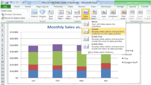
How to format data labels in excel charts. How to Create Excel Charts (Column or Bar) with Conditional Formatting Right-click on any of the columns and pick " Format Data Series " from the contextual menu that pops up. In the task pane, change the position and width of the columns: Switch to the Series Options tab. Change " Series Overlap " to " 100%. " Set the Gap Width to " 60%. " Step #4: Adjust the color scheme. At last, add the final touches. How to Create a Bar Chart With Labels Above Bars in Excel In the Format Data Labels pane, under Label Options selected, set the Label Position to Inside End. 16. Next, while the labels are still selected, click on Text Options, and then click on the Textbox icon. 17. Uncheck the Wrap text in shape option and set all the Margins to zero. The chart should look like this: 18. How to create Custom Data Labels in Excel Charts Two ways to do it. Click on the Plus sign next to the chart and choose the Data Labels option. We do NOT want the data to be shown. To customize it, click on the arrow next to Data Labels and choose More Options … Unselect the Value option and select the Value from Cells option. Choose the third column (without the heading) as the range. Add or remove data labels in a chart - Microsoft Support Add data labels to a chart · Click the data series or chart. · In the upper right corner, next to the chart, click Add Chart Element · To change the location, ...
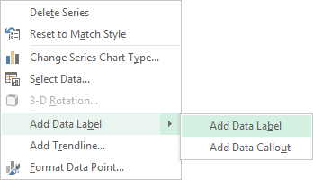
Add a DATA LABEL to ONE POINT on a chart in Excel Click on the chart line to add the data point to. All the data points will be highlighted. Click again on the single point that you want to add a data label to. Right-click and select ' Add data label ' This is the key step! Right-click again on the data point itself (not the label) and select ' Format data label '. excel - Formatting Data Labels on a Chart - Stack Overflow I have written this which deletes every 3 out of 4 data labels so it is easier to read. I would like it though to cycle through all the charts in my workbook and also format the position of the dat... Stack Overflow. About; Products ... Paste Unlinked Excel Chart to Powerpoint. 0. Excel - Programatically get the data used in a chart ... Format Data Labels in Excel- Instructions - TeachUcomp, Inc. Nov 14, 2019 — To format data labels in Excel, choose the set of data labels to format. To do this, click the “Format” tab within the “Chart Tools” contextual ... excel - Formatting chart data labels with VBA - Stack Overflow 1 Answer. Sorted by: 3. You can climb up to a series source range via its Formula property. Since it has the format: =SERIES (,,sheetname!sheetRange,) then you're interested in its "3rd element", if you split it into an array with "," as delimiter. so you can code: Sub FixLabels (whichchart As String) Dim cht As Chart Dim i As Long With Sheets ...
Excel Charts - Aesthetic Data Labels - Tutorialspoint To format the data labels − Step 1 − Right-click a data label and then click Format Data Label. The Format Pane - Format Data Label appears. Step 2 − Click the Fill & Line icon. The options for Fill and Line appear below it. Step 3 − Under FILL, Click Solid Fill and choose the color. How to hide zero data labels in chart in Excel? - ExtendOffice 1. Right click at one of the data labels, and select Format Data Labels from the context menu. See screenshot: 2. In the Format Data Labels dialog, Click Number in left pane, then select Custom from the Category list box, and type #"" into the Format Code text box, and click Add button to add it to Type list box. See screenshot: 3. How to Use Cell Values for Excel Chart Labels Select the chart, choose the "Chart Elements" option, click the "Data Labels" arrow, and then "More Options." Uncheck the "Value" box and check the "Value From Cells" box. Select cells C2:C6 to use for the data label range and then click the "OK" button. The values from these cells are now used for the chart data labels. Excel tutorial: How to use data labels When you check the box, you'll see data labels appear in the chart. If you have more than one data series, you can select a series first, then turn on data labels for that series only. You can even select a single bar, and show just one data label. In a bar or column chart, data labels will first appear outside the bar end. You'll also find options for center, inside end, and inside base. There's also a feature called "data callouts" which wraps data labels in a shape.
How to Add Data Labels in Excel - Excelchat | Excelchat
How to Customize Your Excel Pivot Chart Data Labels - dummies To remove the labels, select the None command. If you want to specify what Excel should use for the data label, choose the More Data Labels Options command from the Data Labels menu. Excel displays the Format Data Labels pane. Check the box that corresponds to the bit of pivot table or Excel table information that you want to use as the label.

Applying basic formatting to charts (graphs) - colors, backgrounds and more
How to Add Data Labels to an Excel 2010 Chart - dummies On the Chart Tools Layout tab, click Data Labels→More Data Label Options. The Format Data Labels dialog box appears. You can use the options on the Label Options, Number, Fill, Border Color, Border Styles, Shadow, Glow and Soft Edges, 3-D Format, and Alignment tabs to customize the appearance and position of the data labels.

Microsoft Excel Tutorials: The Chart Layout Panels
Custom Data Labels with Colors and Symbols in Excel Charts - [How To] Step 4: Select the data in column C and hit Ctrl+1 to invoke format cell dialogue box. From left click custom and have your cursor in the type field and follow these steps: Press and Hold ALT key on the keyboard and on the Numpad hit 3 and 0 keys. Let go the ALT key and you will see that upward arrow is inserted.

32 Data Label Excel - Labels Design Ideas 2020
Add / Move Data Labels in Charts - Excel & Google Sheets We'll start with the same dataset that we went over in Excel to review how to add and move data labels to charts. Add and Move Data Labels in Google Sheets. Double Click Chart; Select Customize under Chart Editor; Select Series . 4. Check Data Labels. 5. Select which Position to move the data labels in comparison to the bars. Final Graph with Google Sheets

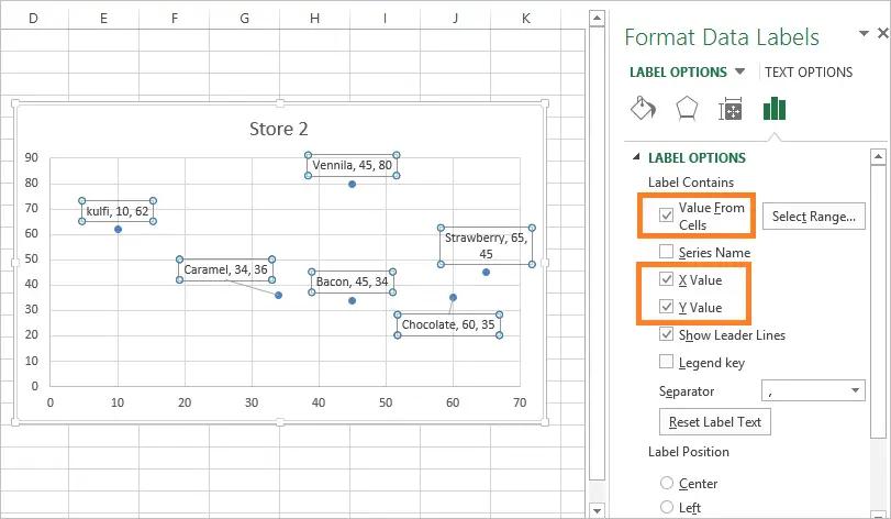
Improve your X Y Scatter Chart with custom data labels
How to Insert Axis Labels In An Excel Chart | Excelchat We will again click on the chart to turn on the Chart Design tab. We will go to Chart Design and select Add Chart Element. Figure 6 - Insert axis labels in Excel. In the drop-down menu, we will click on Axis Titles, and subsequently, select Primary vertical. Figure 7 - Edit vertical axis labels in Excel. Now, we can enter the name we want ...

30 How To Add Label To Excel Chart - Labels Database 2020
Use custom formats in an Excel chart's axis and data labels Right-click the Axis area and choose Format Axis from the context menu. If you don't see Format Axis, right-click another spot. Choose Number in the left pane. (In Excel 2003, click the Number...

Create Custom Data Labels in Excel Charts - YouTube
How to I rotate data labels on a column chart so that they are ... To change the text direction, first of all, please double click on the data label and make sure the data are selected (with a box surrounded like following image). Then on your right panel, the Format Data Labels panel should be opened. Go to Text Options > Text Box > Text direction > Rotate
Add Custom Labels to x-y Scatter plot in Excel - DataScience Made Simple
How To Add Data Labels In Excel | Nabludatel Change position of data labels. Excel provides several options for the placement and formatting of data labels. Source: . Enter field names for each column on the first row. To format data labels in excel, choose the set of data labels to format. Source: superuser.com. The "label options" window will appear.

How to Create Multi-Category Chart in Excel - Excel Board
How to format the data labels in Excel:Mac 2011 when showing a ... Phillip M Jones. Replied on December 7, 2015. Try clicking on Column or Row you want to set. Go to Format Menu. Click cells. Click on Currency. Change number of places to 0 (zero) (if in accounting do the same thing.

Excel Course: Inserting Graphs
How to add or move data labels in Excel chart? - ExtendOffice In Excel 2013 or 2016. 1. Click the chart to show the Chart Elements button . 2. Then click the Chart Elements, and check Data Labels, then you can click the arrow to choose an option about the data labels in the sub menu. See screenshot: In Excel 2010 or 2007. 1. click on the chart to show the Layout tab in the Chart Tools group. See screenshot: 2. Then click Data Labels, and select one type of data labels as you need. See screenshot:

Directly Labeling Excel Charts - PolicyViz
Excel charts: add title, customize chart axis, legend and data labels Click anywhere within your Excel chart, then click the Chart Elements button and check the Axis Titles box. If you want to display the title only for one axis, either horizontal or vertical, click the arrow next to Axis Titles and clear one of the boxes: Click the axis title box on the chart, and type the text.

Microsoft Excel Tutorials: The Chart Layout Panels
Custom Chart Data Labels In Excel With Formulas Select the chart label you want to change. In the formula-bar hit = (equals), select the cell reference containing your chart label's data. In this case, the first label is in cell E2. Finally, repeat for all your chart laebls. If you are looking for a way to add custom data labels on your Excel chart, then this blog post is perfect for you.

Automatically update data labels on Excel chart (Excel 2016) - Stack Overflow
Edit titles or data labels in a chart - Microsoft Support Right-click the data label, and then click Format Data Label or Format Data Labels. Click Label Options if it's not selected, and then select the Reset Label Text check box. Top of Page Reestablish a link to data on the worksheet On a chart, click the label that you want to link to a corresponding worksheet cell.

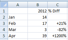
Show Trend Arrows in Excel Chart Data Labels
How to Change Excel Chart Data Labels to Custom Values? Go to Formula bar, press = and point to the cell where the data label for that chart data point is defined. Repeat the process for all other data labels, one after another. See the screencast. Points to note: This approach works for one data label at a time. So if you have a large chart, you are in for a lot of clicks and manic mouse maneuvering.
How-to Add Custom Labels that Dynamically Change in Excel Charts - Excel Dashboard Templates
Creating a chart with dynamic labels - Microsoft Excel 2013
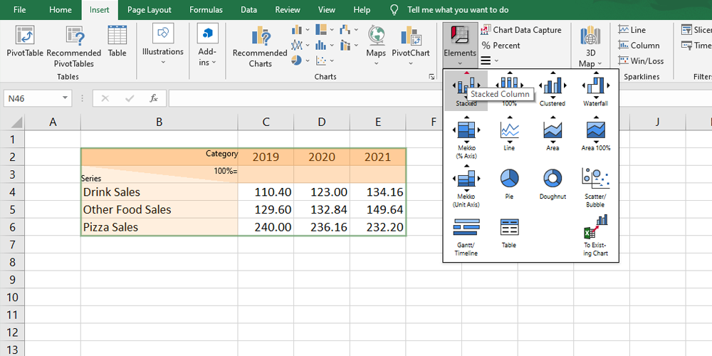
Automate a Think-Cell Chart with Excel Data - Slide Science
Variance Analysis in Excel - Making better Budget Vs Actual charts - PakAccountants.com
Post a Comment for "41 how to format data labels in excel charts"